Planning retirement finances is harrowing; finding reliable, disinterested information is difficult. This paper studies and constructs a portfolio based on a set of formal requirements and analyses its potential performance by back-testing on 20 years of history.
Problem statement and Requirements
Given a single down-payment, construct a portfolio that will generate a retirement pension.
A stipend will be withdrawn the beginning of each year. The amount will increase by 1.3% p/a to compensate for the average inflation in Switzerland.
The portfolio’s life shall exceed 30 years.
Objectives
- The risk of total loss is minimised.
- The portfolio shall be as resilient as possible to market turmoil.
Constraints
- Instruments. Given the problem statement, the only viable instrument is shares.
- Bonds cannot produce the required revenue.
- Derivatives are subject to default by the writer.
- Funds have a risk of default by the managing entity and their performance is predicated by fees.
- Real-estate companies (as opposed to funds) that actually possess all their properties are acceptable because they are backed with physical property.
- Currency. CHF only; forex risks are unacceptable because every currency has lost value against the Swiss Franc in the last 20 years.
- Geography. The shares shall be in Swiss companies domiciled in Switzerland.
- Debtor Diversity: No single company shall represent more than 5% of the portfolio.
- Industry Diversity: No single industry shall represent more than 5% of the portfolio.
Deliverables
- A set of objective criteria for stock picking that fulfils the constraints.
- Based on these criteria, a basket of desirable shares in which to invest.
- Buying, re-balancing and selling strategies.
- An estimate of the stipend percentage range.
- An analysis of the basket’s performance, by back-testing on historical data 2000-2019, which will determine:
- The buffer that needs to be kept to maintain yearly payments, so as not to be obliged to sell at an unfavourable moment.
- The portfolio’s probable behaviour in worst-case scenarios (e.g. entering the market just before a stock-market crash).
- Situations in which the portfolio’s life might be compromised and mitigating actions.
Selection Criteria
An ideal company would have a healthy balance sheet, exhibit constant growth and lose no value during a stock-market crash. Such companies do not exist, however amongst the 40-odd financial ratios available, 3 are particularly useful to filter out desirable candidates.
- The Sortino ratio, a downside variant of the Sharpe ratio, is a strong predictor of companies that have the desired kind of behaviour.
- The Quick Ratio, whilst dependent on the industry, generally demonstrates that a company has had the foresight to keep enough cash on hand to weather difficulties.
- Resistance to turmoil, which can be assessed by observing the stock’s behaviour during a stock-market crash. It consists of two associated components:
- Resilience. The percentage value remaining after a crash.
- Recovery. The period of time before the stock re-attains its pre-crash value.
Graphically:
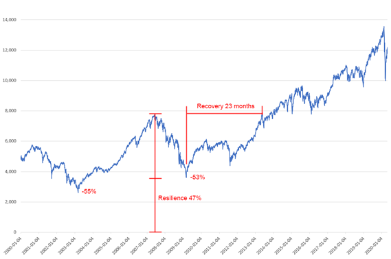
Ideal shares will have a resilience close to 100% and a short recovery.
(This graph is in fact the SPI and there were two major crashes. The latter is used as it is more recent. Thus, the SPI has a resilience of 47% and a recovery of 23 months).
Stock Selection
An initial selection is performed where companies will be scored using a decision matrix with 4 components outlined above:
- The Sortino ratio, weight 20%.
- The Resilience, weight 30%.
- The Recovery, weight 30%.
- The Return (growth plus dividend), weight 20%.
Note: The gold standard for expressing portfolio returns is the CAGR (Compound Average Growth Rate) but as it is calculated using solely a start and ending value, it is sensitive to the end-points:
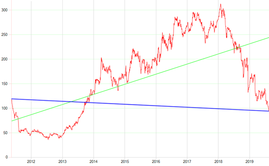
This extreme case has a CAGR of -0.1% (the blue line) but over the entire period its global trend is positive (the green line, a least-squares linear fit).
Shares’ growths will be measured using the slope of the green line, expressed as a percentage of the average value, in this example 12%. The CAGR will also be calculated and used as a cross-check for cases like this.
From this subset a manual review will determine the companies finally chosen (judgement is required for the Quick Ratio, which has different meanings for each industry).
Universe
The initial instrument universe is the SPI and Swiss Real-Estate companies. Of the 215 SPI shares, 205 are quoted in CHF and totally domiciled in Switzerland. Of these, 82 and have been quoted continuously since 2000 and show positive returns.
Duplicate shares (e.g. Lindt N and Lindt PS) are be eliminated by the lowest score.
To meet the diversity constraint, a single stock with the best score of each industry segment is retained.
Selected shares
After applying the criteria and manual selection 21 shares remain:
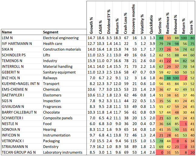
These will constitute the proposed portfolio. The benchmark is the SPI.
Rejects
The remaining shares were eliminated because:
- Railways. Despite their high scores, TITL BN BERG and JUNGFRAUBAHN HLD both have their entire infrastructure in one location. They were dropped in favour of BVZ HOLDING, which is significantly more diversified.
- Foods. NESTLE scored lower but was preferred over BELL AG, which is not entirely Swiss and focussed on a single product line, meat. GROUP MINOTERIES has poor returns.
- Chocolates. BARRY CALLEBAUT has a slight edge over LINDT and VILLARS.
- The remainder due to insufficient resilience and/or recovery.
Weighting
The SPI index components are weighted by companies’ market value, as the aim is to assess the performance of the total CHF amount invested in the market.
On the other hand, an investor’s components are chosen to diversify risk; it is thus undesirable to give more weight to any particular company as this would proportionally increase risk for that component. Consequently, the portfolio will be built with equal CHF amounts of each stock.
Performance Analysis
The baseline comparison consists of comparing the portfolio against the SPI and SMI, normalised to 100 on the 1st of January 2000:
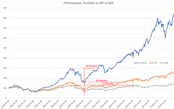
Despite the impression due to the scale, all three lost ~55% in the 2007-2008 crash.
The portfolio recovers much faster (20 months), than the SPI (50 months) or the SMI (73 months).
Note: The SPI’s CAGR over the last 30 years is 9.89%.
Buffering
Selling shares to obtain cash for stipends is undesirable after a stock market crash, as their value will be down by some 55%. There is thus a requirement for a cash buffer to avoid such sales.
The portfolio recovers from a crash in some 20 months. Assuming that a stock-market crash occurs about once a decade, there will be two or three stock market crashes during the portfolio’s lifetime.
As the first crash can occur at inception, the minimum buffer is 2 year’s stipends. Assuming that the stipend is low enough to allow the portfolio to grow during the first half of its life, it may not be necessary to buffer for subsequent crashes.
Buffering with cash is costly with the current -0.7% negative interest. An attractive alternative is to use Real-Estate, which offers more modest growth but suffers much less in troubled markets. Of the 31 Real-Estate companies quoted on SWX, only 5 meet the criteria:

Their worst-case behaviour is a loss of ~15% and a recovery of 11 months, which is an acceptable level of risk given their average growth of 6.6%. (A 15% loss is covered by growth if the first crash occurs no earlier than 27 months after inception.)
This buffering strategy will be tested in the simulation.
Buying, Re-balancing and Selling strategies
Buying
Of the 116’213 price changes of the members of the portfolio in the past 20 years, the average change was +0.0056 CHF. It follows that given the choice of buying today or waiting until tomorrow in the hope that the price will go down, it is logical to buy today (with an appropriate limit to avoid getting executed ‘high’ in the day).
This can by improved by observing a stock’s historical random walk to determine the chances of buying at a lower price over some period. For a given stock, for each day in the history, determine how often a price fall of at least X% occurred in the N following days (here, N=60):
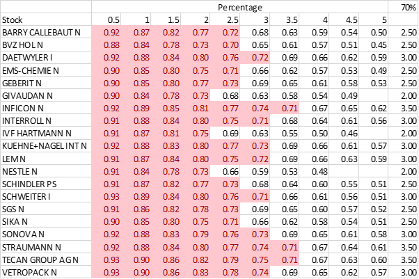
Thus, if I want to buy Barry Callebaut, there is a 72% chance that it will fall by 2.5% in the next 60 days. Intuitively, sought-after shares (Givaudin, IVF Hartmann and Nestlé) are less likely to fall, so the limited order will need to be closer to the current price. Conversely, more volatile shares (Straumann and Tecan) are more likely to be had at a larger discount.
The buying strategy is thus to place limited orders at a discount of the percentage which meets the chosen chance of success. I implemented this strategy on the 2nd of October 2020. On the 20th of November, I had acquired 19 out of the 20 stocks at an average discount of 2.3% below the October 2nd prices, so this strategy works (except for Kühne & Nagel, which never fell 3% during the period).
Re-Balancing
The average cost of a transaction is about 0.85%, so the re-balancing cost is 1.7% of the position. This churning must be weighed against the hypothetical gain obtained by improved diversification.
It makes more sense to sell smaller fractions of multiple positions rather than entire positions, as the difference in transaction fees is negligible (0.825% for transactions over 50’000 versus 0.9% for those below 50’000).
Selling
The stipend pay-out will be made each year, using the dividends and sales as necessary. The simulations determined that the optimal rules for selling are:
- When the market has fallen over the preceding year, prefer to sell real-estate otherwise sell shares (avoid selling shares at a poor price).
- Select the 5 shares that have the highest growth in the last 12 months (5 was determined empirically).
- Choose the two largest CHF positions.
- Sell half the necessary amount of each of the two positions (to minimise unbalancing).
If a sale would represent more than 90% of the position, sell the entire position (to avoid subsequent odd-lot trades.
Simulation
A simulator was built to perform the back-testing. It operates as follows:
The simulation is initiated by:
- Setting the clock to the start date.
- Depositing CHF 1’000’000 in the account.
- Immediately paying the stipend, proportional to the time remaining in the current year.
- Use the remaining cash to populate the portfolio with shares and real-estate.
Then, repeatedly:
- Advance the clock to 31st of December.
- Calculate the dividends from the current positions and remove 35% withholding tax (which is written off). Credit the portfolio cash with the remaining 65%.
- Pay-out custodian fees of 0.35% of the portfolio’s current market value.
- Advance to 1st of January.
- Increase the stipend by the rate of inflation.
- Sell a sufficient amount of positions to make the cash greater than the current stipend.
- Pay-out the stipend (or declare failure if there is insufficient cash).
Finally, calculate the P&L and various statistics.
Transaction fees are applied at the rates for UBS Online Banking. The rate varies by transaction size, about 0.85%. Other brokers / custodians charge significantly less.
SWX fees and Stamp Duty are also deducted.
Results
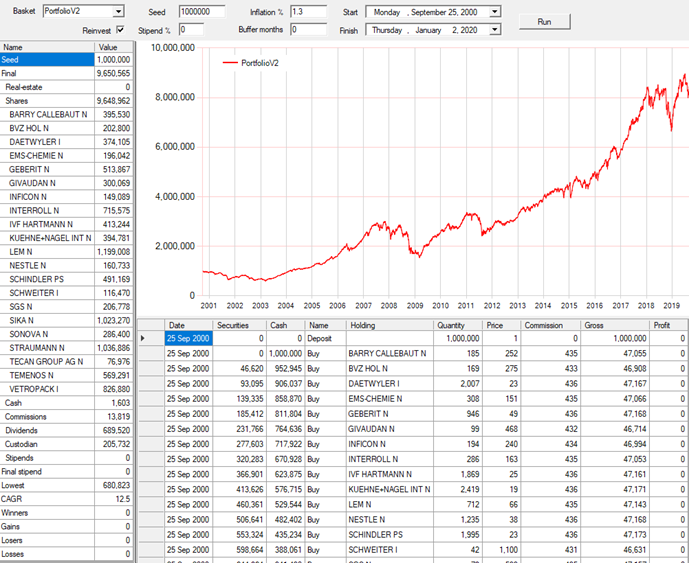
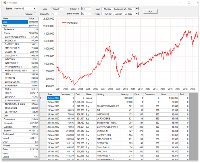
A typical simulation produces the following:
Discussion
This is a worst-case, the 2000 stock-market crash commenced on the 25th of September 2000. The other worst case, starting on the 15th of October 2007, produces almost identical results.
The stipend is 7.2%, CHF 72’000 on the first year, increasing to 92’026 after 20 years.
There are practically no sales at a loss.
The portfolio’s costs are 95’606 ÷ 20 years = 4’780 per year = ~0.5%. This could be significantly reduced by using a less expensive broker / custodian, e.g. SwissQuote.
The total stipends amount to 1’632’512 for an initial investment of 1’000’000.
The portfolio’s final value is just over double the initial deposit.
The portfolio has a CAGR of 3.8%, despite the stipend withdrawals.
The asset allocation remains moderately well balanced at the end of the simulation, the 21 initial companies all remain.
Determining the ideal buffer
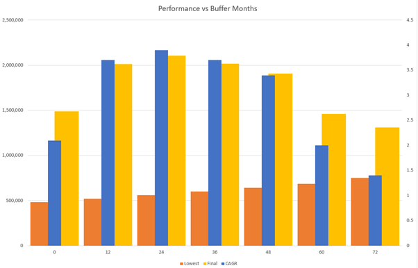
Simulations were performed for varying buffer sizes from 0 to 6 years. Whilst increasing the buffer has a positive effect on the portfolio’s lowest value, the final portfolio value and the CAGR are affected negatively. It transpires that a buffer of ~30 months is optimal:
Maximum stipend
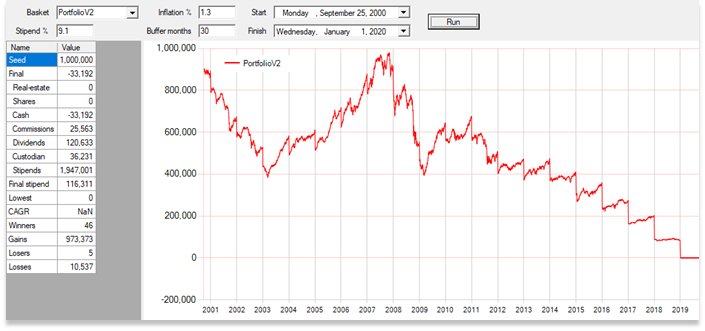
The portfolio fails (again, starting on worst-case 25/9/2000) at a stipend of 9.1%:
Ideal stipend
The chosen stipend is a function of the investor’s appetite for risk. With a stipend of 7.2% (the typical simulation above), the portfolio final value was 2’056’468 with a CAGR of 3.8%.
Decreasing the stipend to a more conservative 6% increases the final value to well over 3’000’000 with a CAGR of 6.2%:
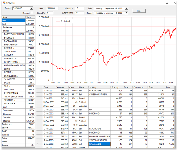
Observe the transactions after the 2000 stock-market crash, where real-estate buffer is sold rather than stocks, until 2003 with the Givaudan sale.
Unfavourable situations
It is well-known that past performance is not a predictor for the future and a simultaneous stock-market and real-estate crash remains possible. Unforeseeable black-swan events will certainly happen in the incoming 30 years.
That said, most of the selected companies are manufacturers that have an established niche, producing tangible goods. All have a healthy balance sheet and have been well-managed for decades; the risk of total loss is thus extremely small.
Conclusion
The designed portfolio, implemented with a buffer of 30 months and a stipend of 6% meets the requirements with minimal risk.
Post-Scriptum
The same portfolio, run with neither stipends nor buffering and re-investing the dividends, starting on the pre-crash worst-case in September 2000, has the following behaviour (a CAGR of 12.5%):
