TLDR: Results . Lessons learned . Summary & Conclusions . Quick-start guide
I am building an autonomous lawnmower which needs to know its position precisely – in the order of centimetres. Standard GPS is an order of magnitude too coarse and until recently, all flavours of differential GPS were very expensive. This changed last year when UBlox released the C94-M8P with a price tag of €359 for a complete solution. The announcement said:
The NEO-M8P module series introduces the concept of a “Rover” and a “Base Station”. By using a correction data stream from the Base Station, the Rover can output its relative position with stunning cm-level accuracy in good environments.
An old dog, I was wary of “in good environments”. That RTK is capable of centimeter accuracy when stationary and with a horizon-to-horizon view of the sky, I have no doubt; but what about in a less GPS-friendly environments? This article is the result of real-life testing in my garden, cluttered by surrounding buildings and vegetation..
Objectives
My aim was to establish whether or not the UBlox solution would be sufficiently accurate for my mower,
in particular how would it perform in less-than optimal conditions, so I devised a series of experiments, which I have named for the purposes of this discussion.
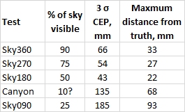
- Open. Stationary for 24 hours in the middle of the lawn, with a decent view of the sky. A base-line test to determine the system performance.
- Sky270. The receiver is next to the corner of a building, 90° of sky are obscured.
- Sky180. The receiver is close to a wall of a building, 180° of sky are obscured.
- Sky090. The receiver is in a corner of a building, 270° of sky are obscured.
- Canyon. The receiver is between two buildings with a heavy tree canopy, most of the sky is obscured.
- Mobile. The receiver is moved around the garden, stopping for 10 seconds at a known location in each of the previous tests.
Tests 2-6 are performed for an hour. As described later, I discovered that the receiver needs 25-30 minutes to settle on a solution and these data were removed.
All the tests are made with the antenna 54cm from the ground.
Test setup
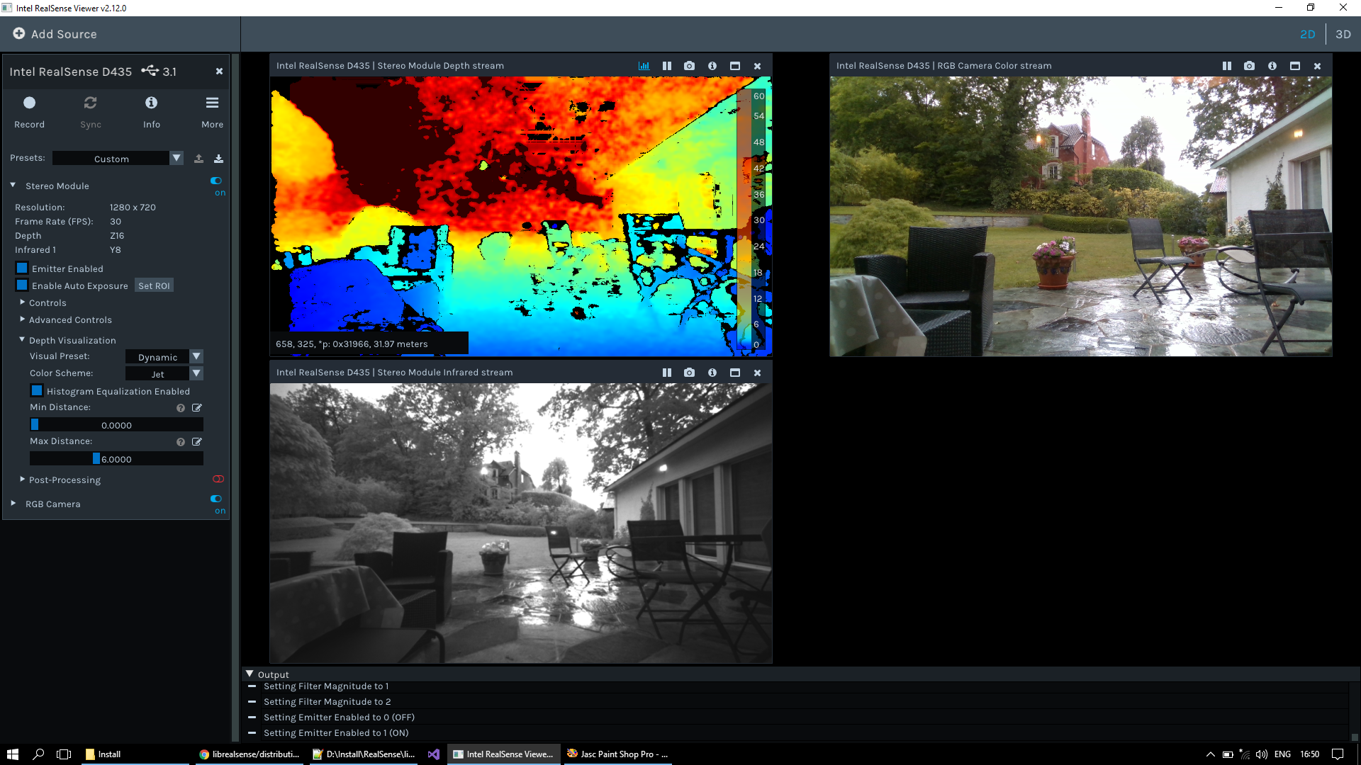
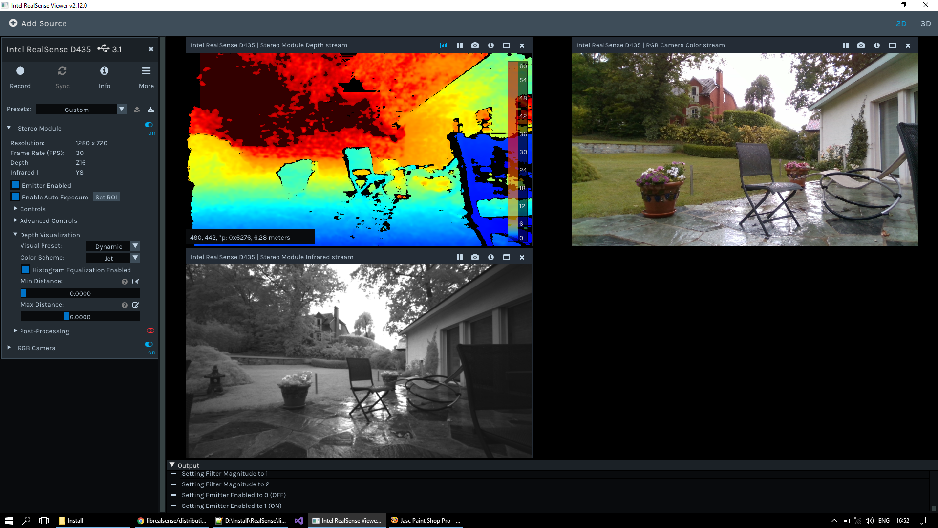
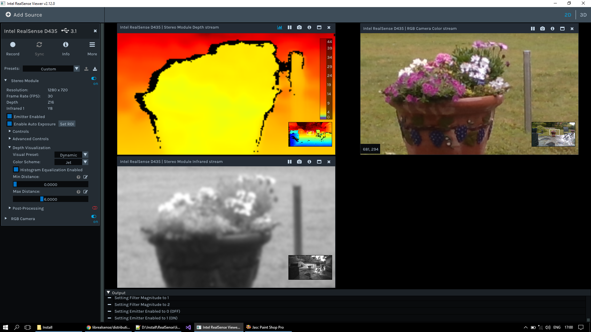
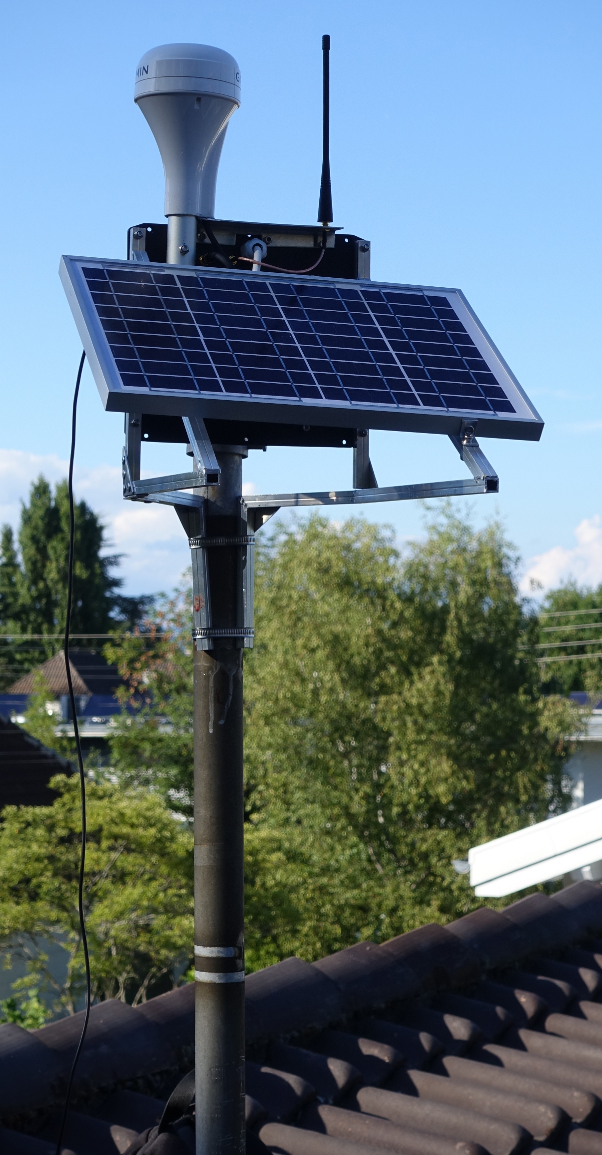
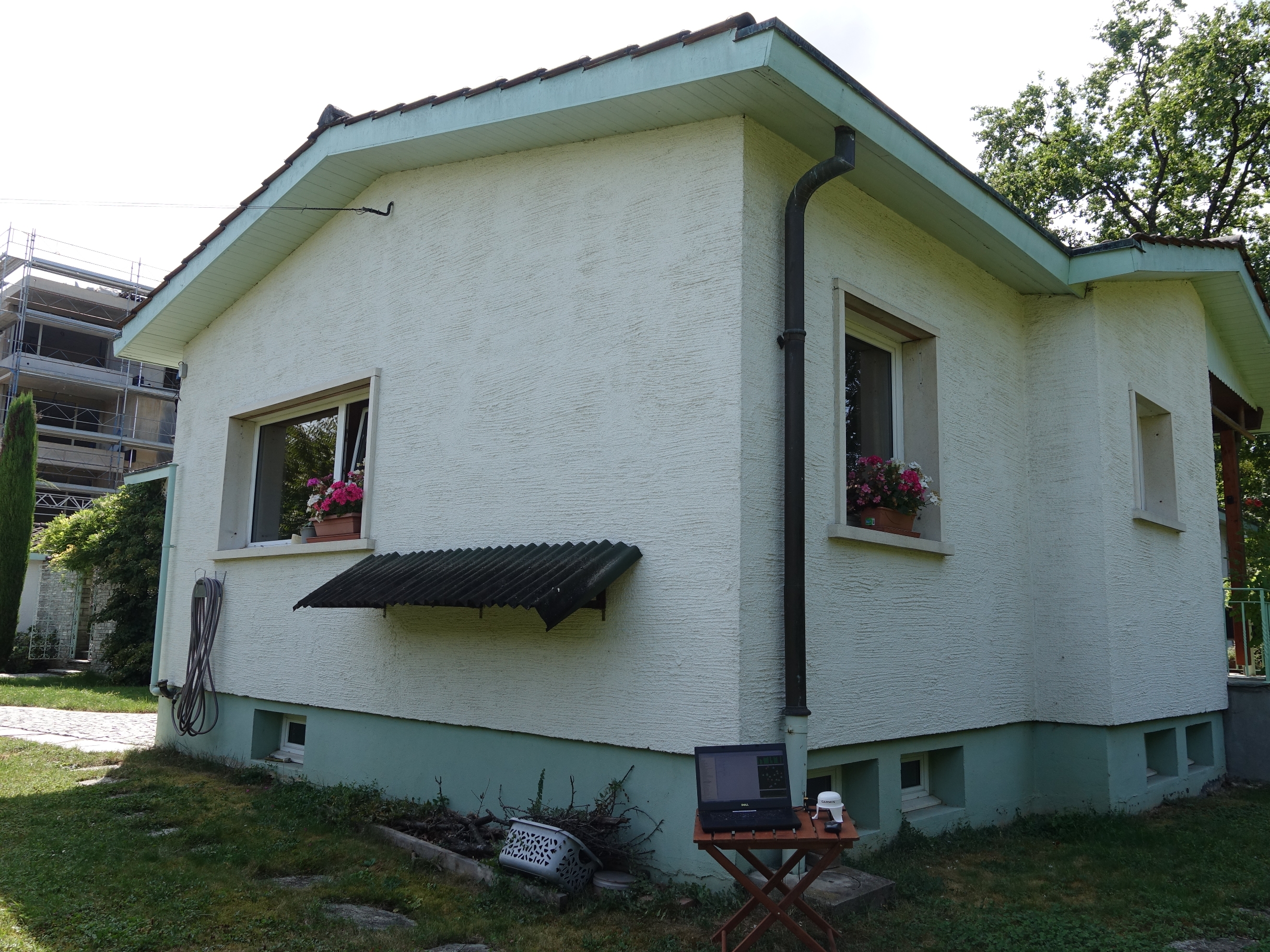
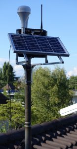
I built a rooftop base station
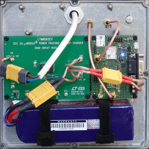
powered by a solar cell with an MPP charger, the DC1621A evaluation board based on the LTM8062 chip from Linear Technology. As I had no idea how much power the C94-M8P would need – after all it has a UHF transmitter – I opted for a 10Ah 2S Lipo. On the left we have the DC1621A, on the right the UBlox board and the battery below. There’s a cell-balancer and packets of silica gel tucked behind the DC1621A. After verifying that every was working correctly, I mounted it on my roof:
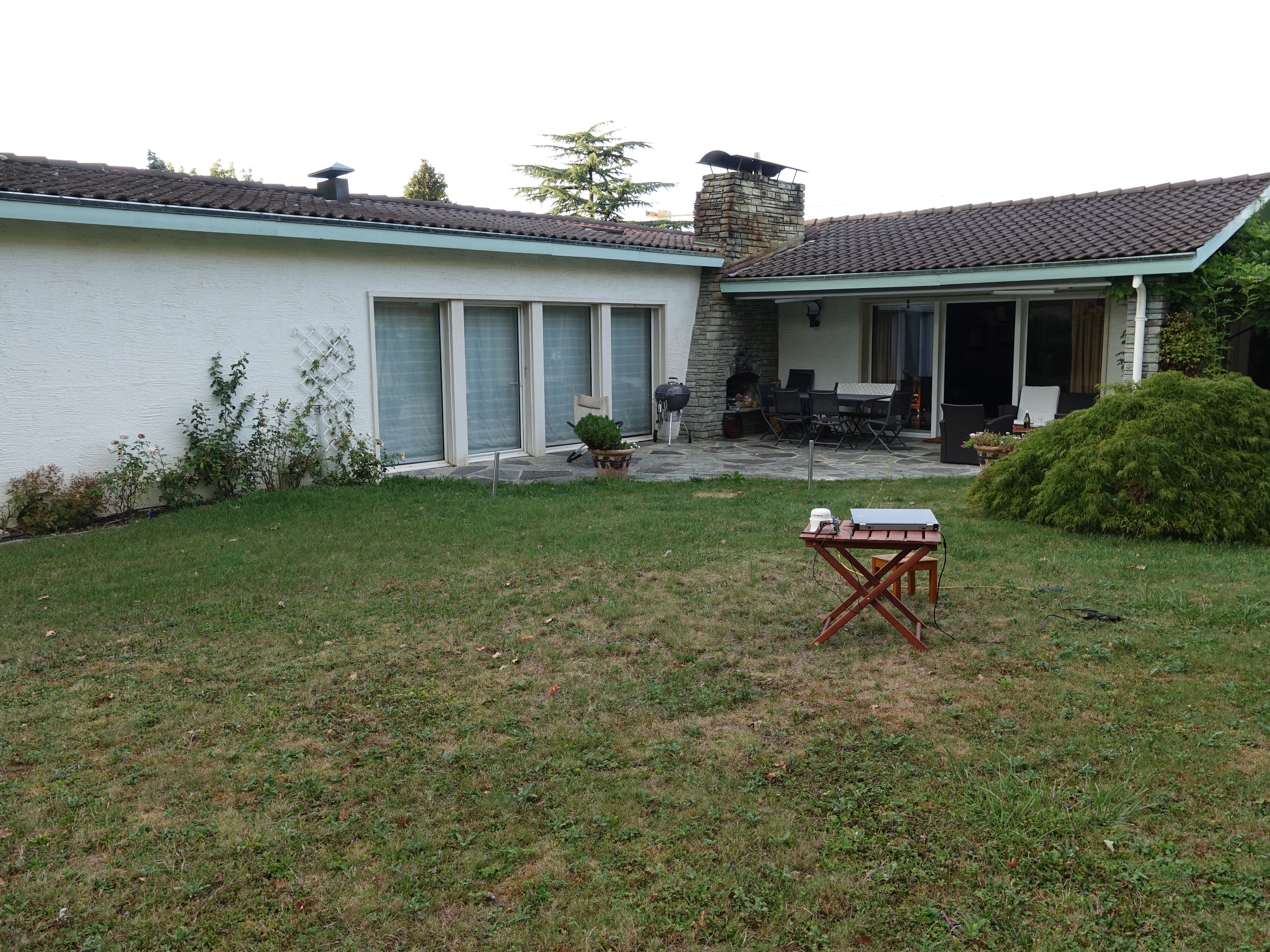
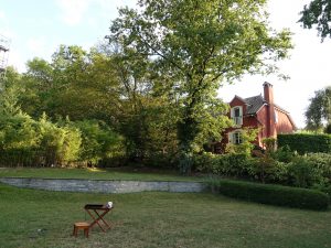
My rover was simply a low table in the garden, with the antenna 54cm off the ground.
The rover’s signature is
In what follows, I am focussed solely on horizontal position – the X, Y values; I ignore altitude as it is only relevant for surveying and aviation.
All my calculations were performed in 64-bit floating point which gives ~15 decimal digits of precision.
The raw GPS data from the receiver contains latitude/longitude values. To convert these into distances I use Vincenty’s formula. I validated my implementation against 500’000 known distances, which are precise to 0.1µ metre.
Outputs
Each test produces 5 results.
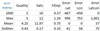
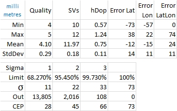
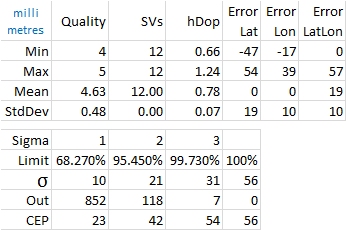
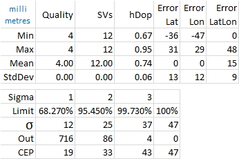
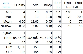
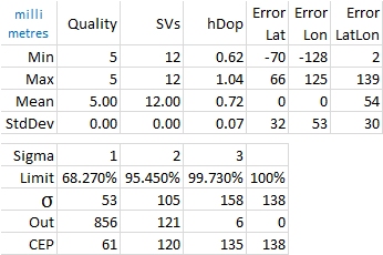
1. Summary statistics
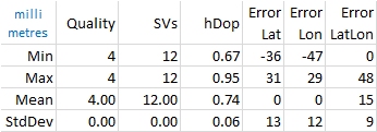
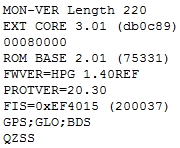
Quality (the NMEA term) is the type of Fix that the GPS currently has. Possible values are:
- Autonomous GNSS
- Differental GNSS
- 3D fix
- RTK Fixed
- RTK Float
It is worth noting that the ‘best’ fix is 4.
SVs is the number of satellites in view. I configured the rover UBX-CFG-NMEA to high precision mode (to output 9 digits of precision on latitude and longitude) and as a result considering mode is disabled. It is unclear whether satellites-in-view is those seen or those actually used.
hDop is the horizontal dilution of precision created by the constellation geometry.
ErrorLat is the distance in millimetres from the average centre of all the readings. Similarly ErrorLon.
ErrorLatLon is Euclidean distance from the measured point and the averaged centre of all the readings.
The ErrorX values are calculated using Vincenty’s Formulæ.
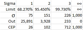
2. Error statistics
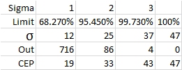
Limit is simply a reminder of the percentages associated with the number of standard deviations.
σ is the standard sigma calculation, the square root of the variance.
Out is the actual number of measurements that exceed the CEP below.
CEP is obtained by finding the number of samples ‘Out’ which exceed the limit %.
The difference between σ (a statistical calculation) and CEP (the true value for the data set in question) is readily explained: The statistical σ is valid only when the data are normally distributed (a Gaussian). Even over 24 hours, GPS readings are not Gaussian because the average is not stationary. Disraeli’s quip remains as true as ever.
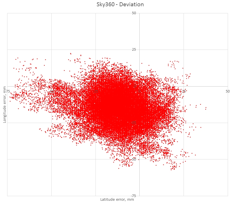
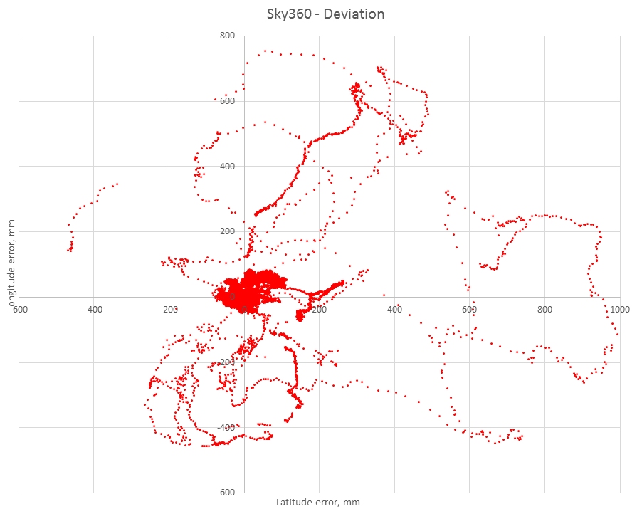
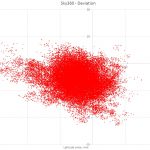
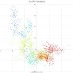
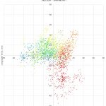
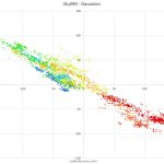
3. Deviation map
An X-Y plot of ErrorLat horizontally against ErrorLon vertically:
A point’s colour indicates its age as hue corrected for the human eye. First blue, then green, yellow, orange and finally red.
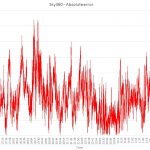
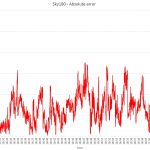
4. ErrorLatLon over time
The Euclidean distance from the average centre to the measured point, in mm, over time:
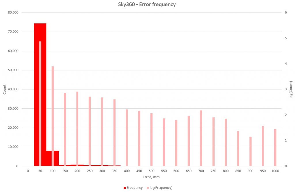
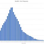
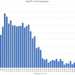
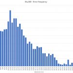
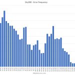
5. Histogram
The number of errors at each bucket of the Euclidean distance from the average centre:
Test results
Open test
Sky visibility is typical for a residential area. To the north and west a single-storey building
The receiver, antenna and PC are on a low table in the foreground.
To the east, a 4-storey building (actually 3-storey but on higher ground)
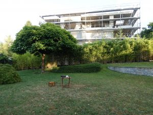
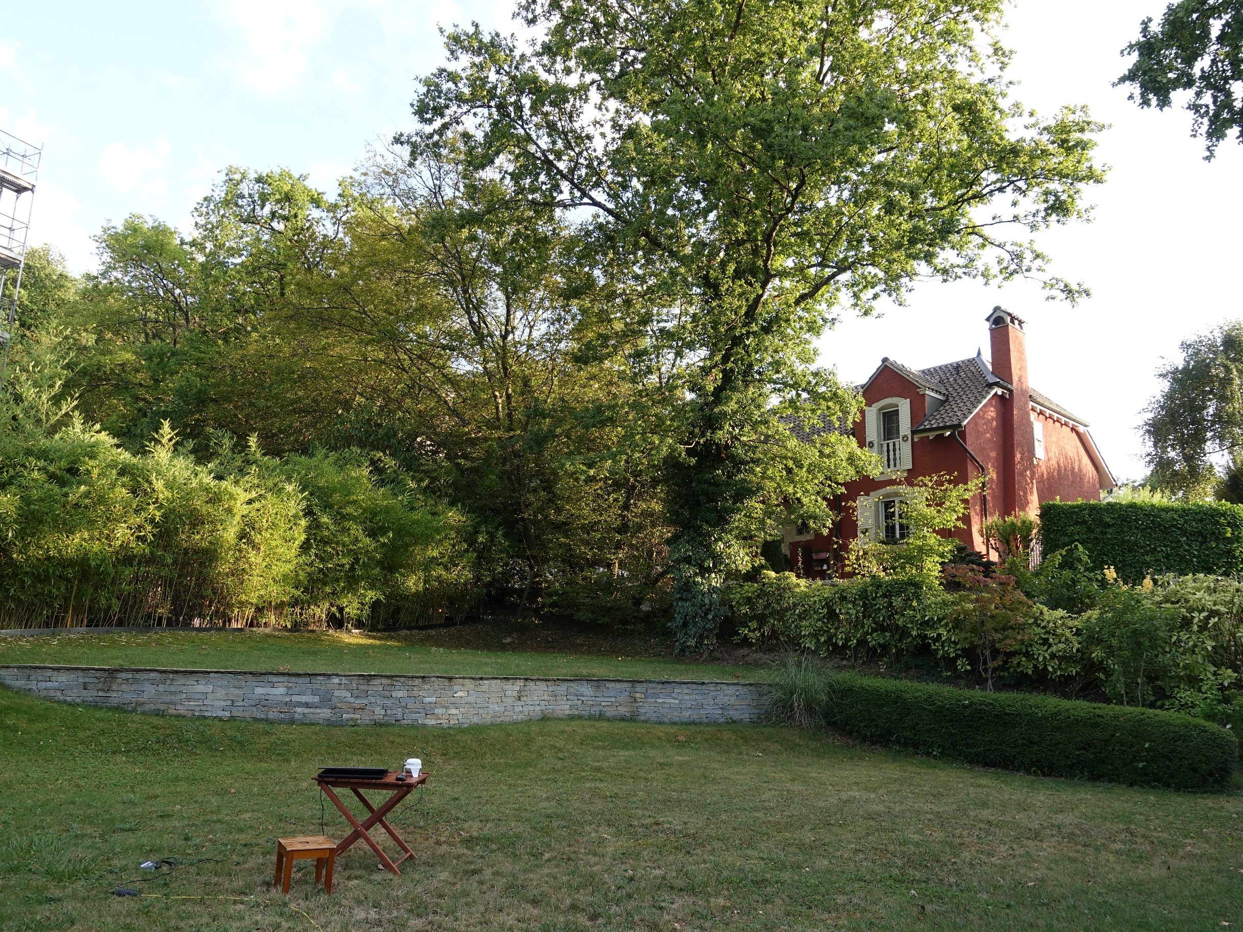
To the south and west, mature oak trees and 2-storey houses

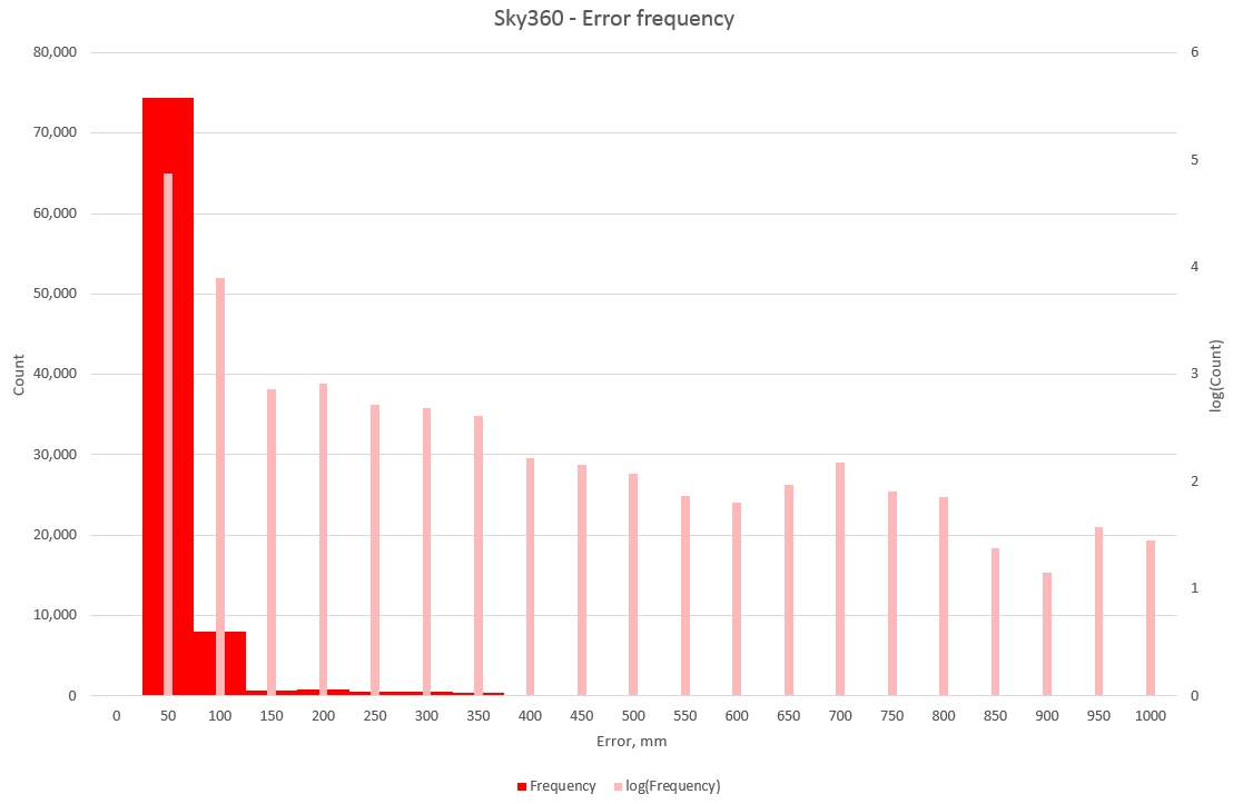
The receiver is in Fixed mode 71% of the time.
The 3σ CEP of 712 mm is surprisingly high and this is visible both in the deviation map:
and in the histogram (I have added log(Count) overlayed on Count to show the long tail more clearly):
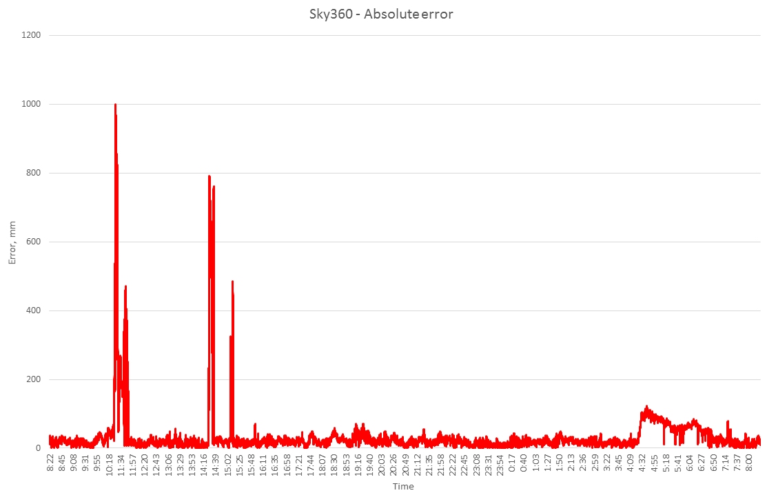
The problem occured mid-morning and early afternoon:

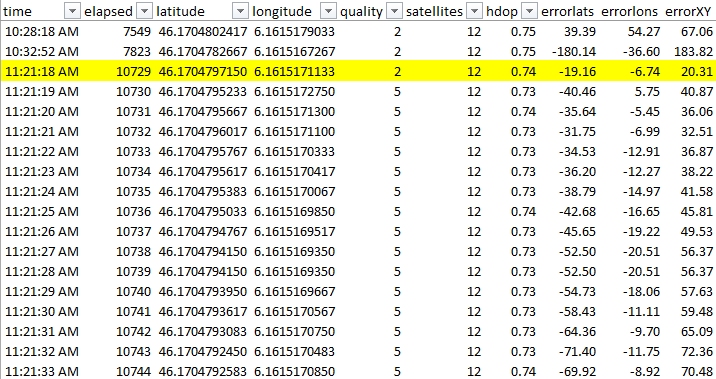
The cause appeared to be due to receiver occasionally losing the RTK solution. To analyse this I zoomed in on the first occurrence and plotted the absolute error along with the Fix. 3D=2, Fixed=4 and Float=5. To highlight the differences, Fixed errors are green, Float errors are blue and 3D errors are red. Notice that the vertical scale is logarithmic:
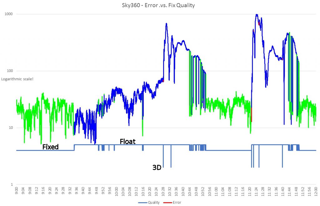
At 10:28:18 and 10:32:52 the receiver switches for one measurement from Float to 3D. The same thing happens at 11:21:18:
and in both cases takes some 20 minutes before settling down.
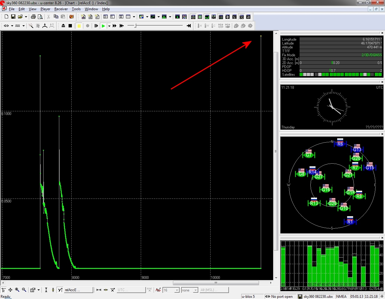
The replay in ucentre shows nothing untoward at the instant of the loss:

I note that 20 minutes is the time that it takes the receiver to lock on cold start (details in Lessons Learned below) and postulate that momentary interference can cause a complete loss of the solution.
There were 4 such events in the 24-hour test. 4 in 86’400 = 1 in 21’600; a frequency less than 4σ, so I sought an explanation.
On the weekend of the tests there was an airshow nearby with several passes of military aircraft in formation. One can reasonably assume that 6 fighters at low altitude produce vast quantities of electromagnetic radiation and I imagine that military RF applications care little about the interference that they generate. Furthermore, the dropouts only occurred during the day, when the aircraft were flying, so I decided that they were the most likely cause. Consequently I decided to use a subset of the data with these events excluded. I also excluded the noisier data as of 04:32 in the morning, on ‘benefit of the doubt’ reasoning, for want of an explanation. The results then become:
Which is what I expected and much more reasonable.
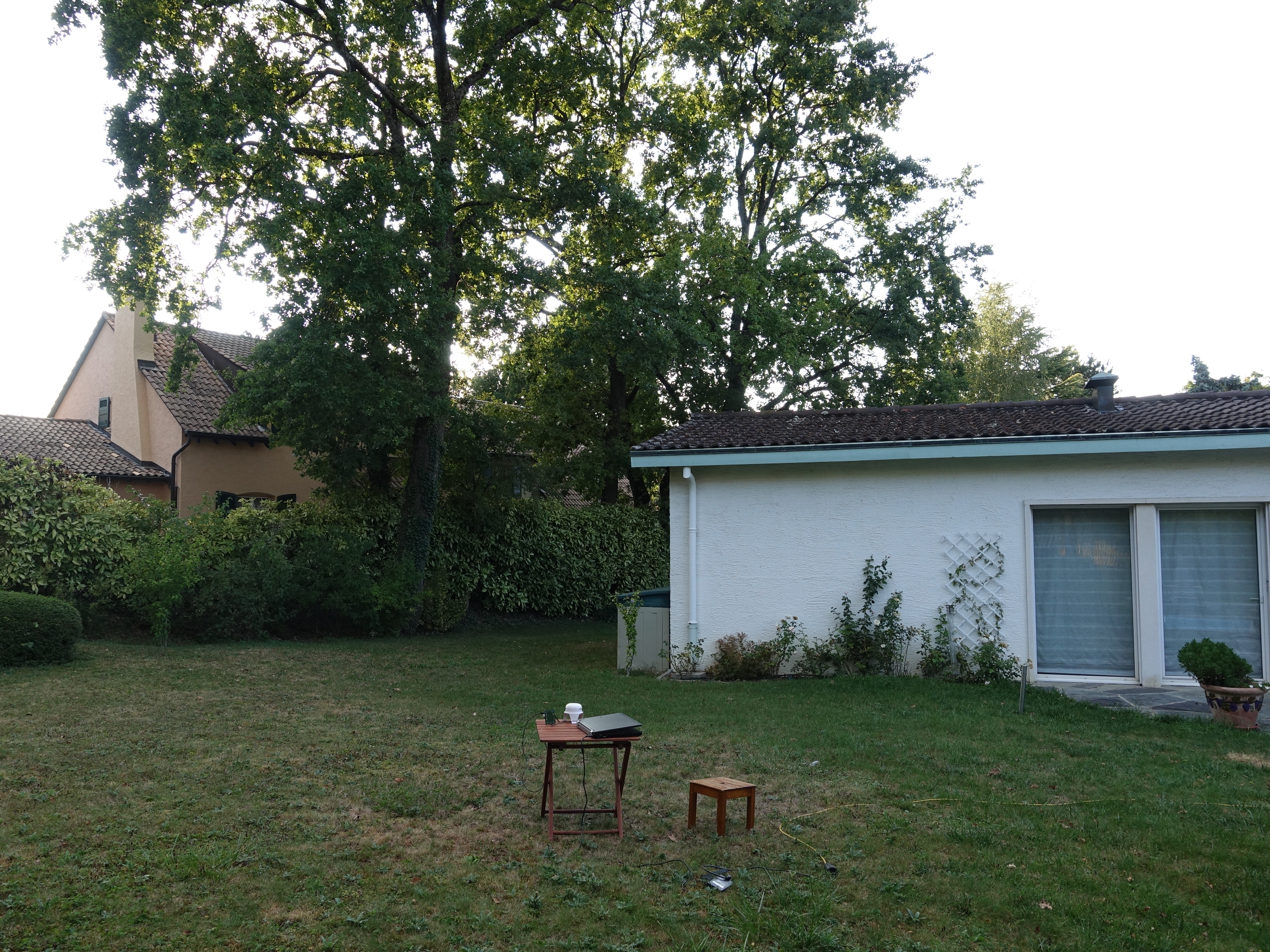
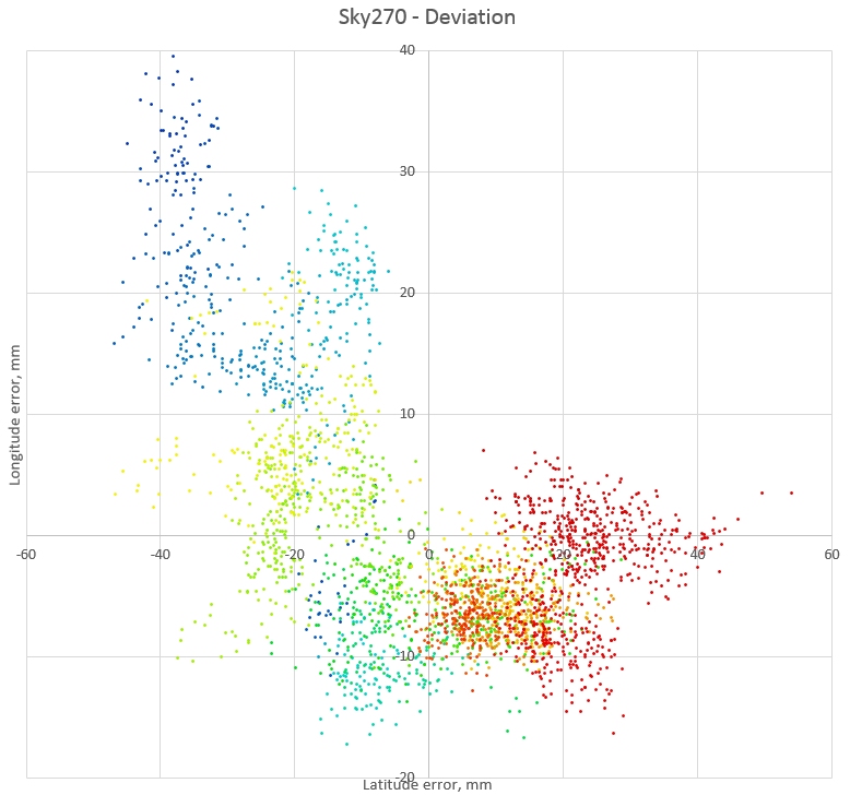
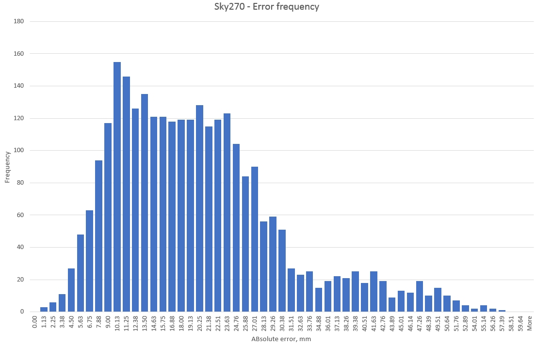
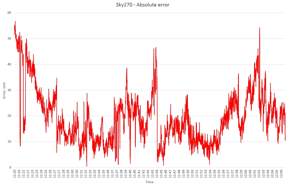
Sky270 test
The receiver is against the NW corner of the house, 90° of obscured sky.

The receiver is slightly more in Float rather than Fixed (4.63 average quality). The 3σ CEP is 54 mm.
There is significantly more longitude error than latitude.
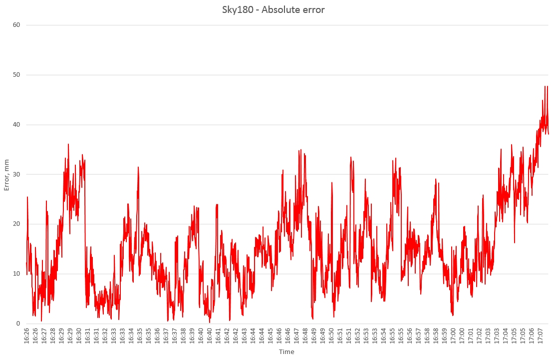
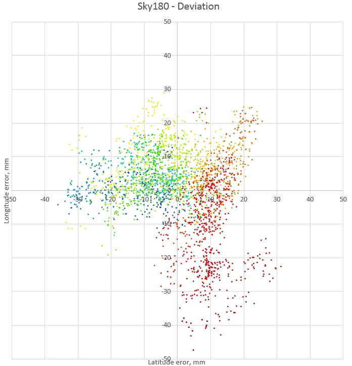
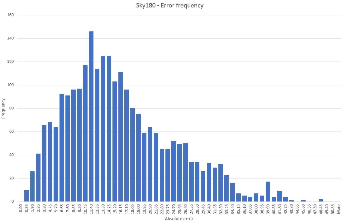
Sky180 test
The receiver is near the NW wall of the house, half the sky is obscured.
The receiver is continuously in Fixed mode. The 3σ CEP is 43 mm.
The histogram has longer tails due to the less favourable constellation geometry (practically no SVs to the SE):
The CEP is better than the Sky270 test, where only 90° of sky were obstructed. I attribute this to the fact that due to the lay of the land, the angle of the apex of the house is much larger when viewed from a corner. Additionally the sky view away from the house in this position is a little more cluttered.
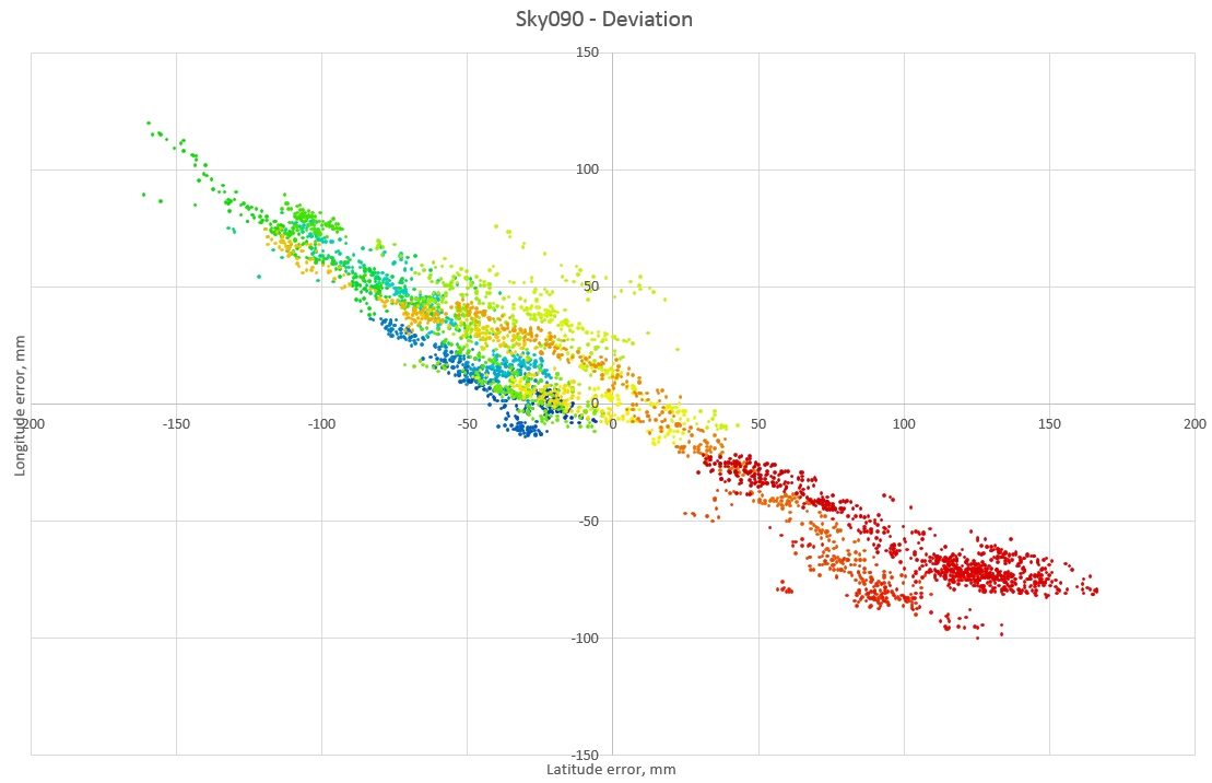
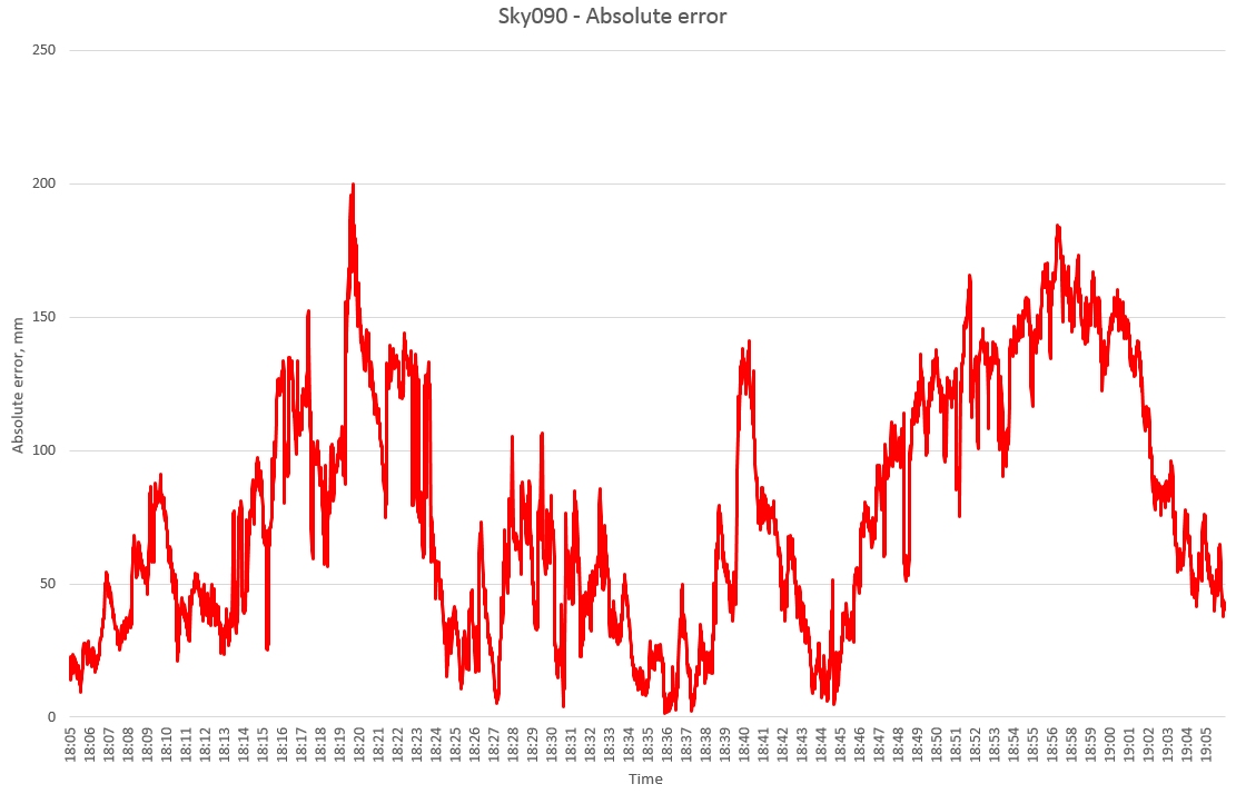
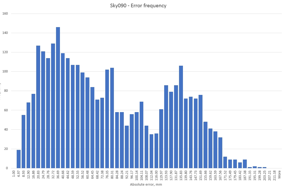
Sky90 test
The receiver is in a corner of a building, facing SW, 270° of sky are obscured.
The receiver is in Fixed mode for the whole hour. The 3σ CEP is 185 mm.

The deviation shape clearly reflects the SW direction of the corner.
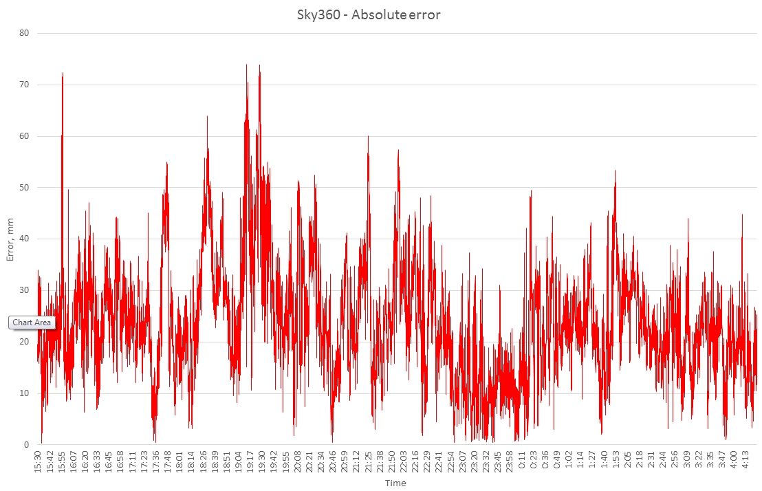
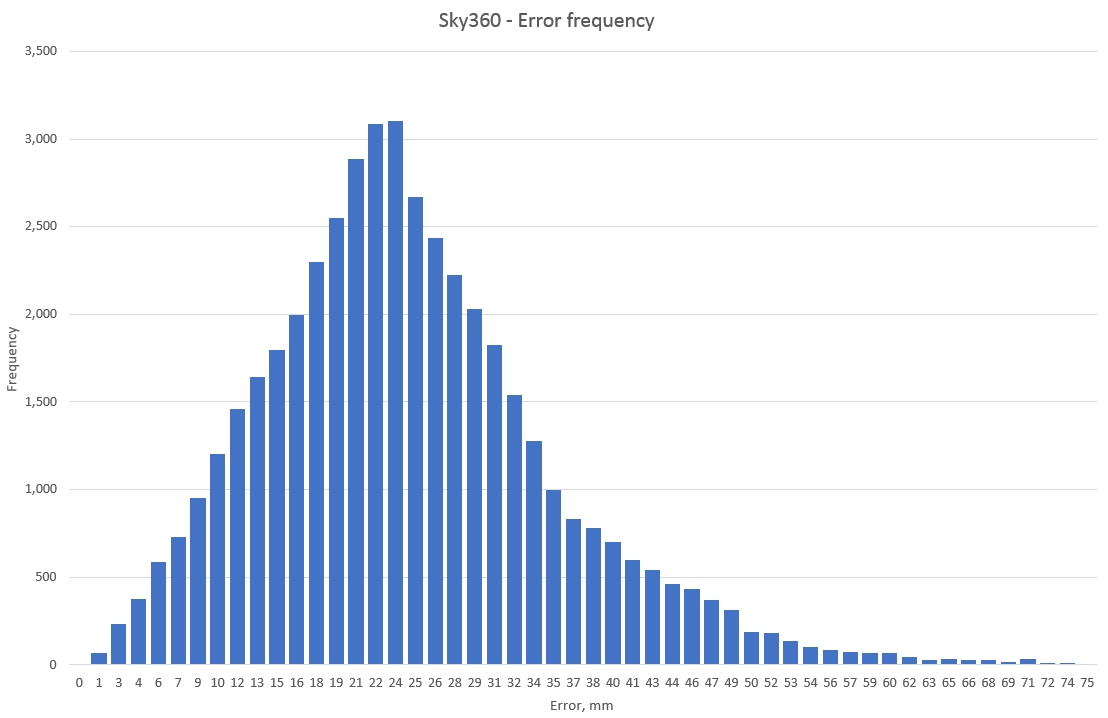
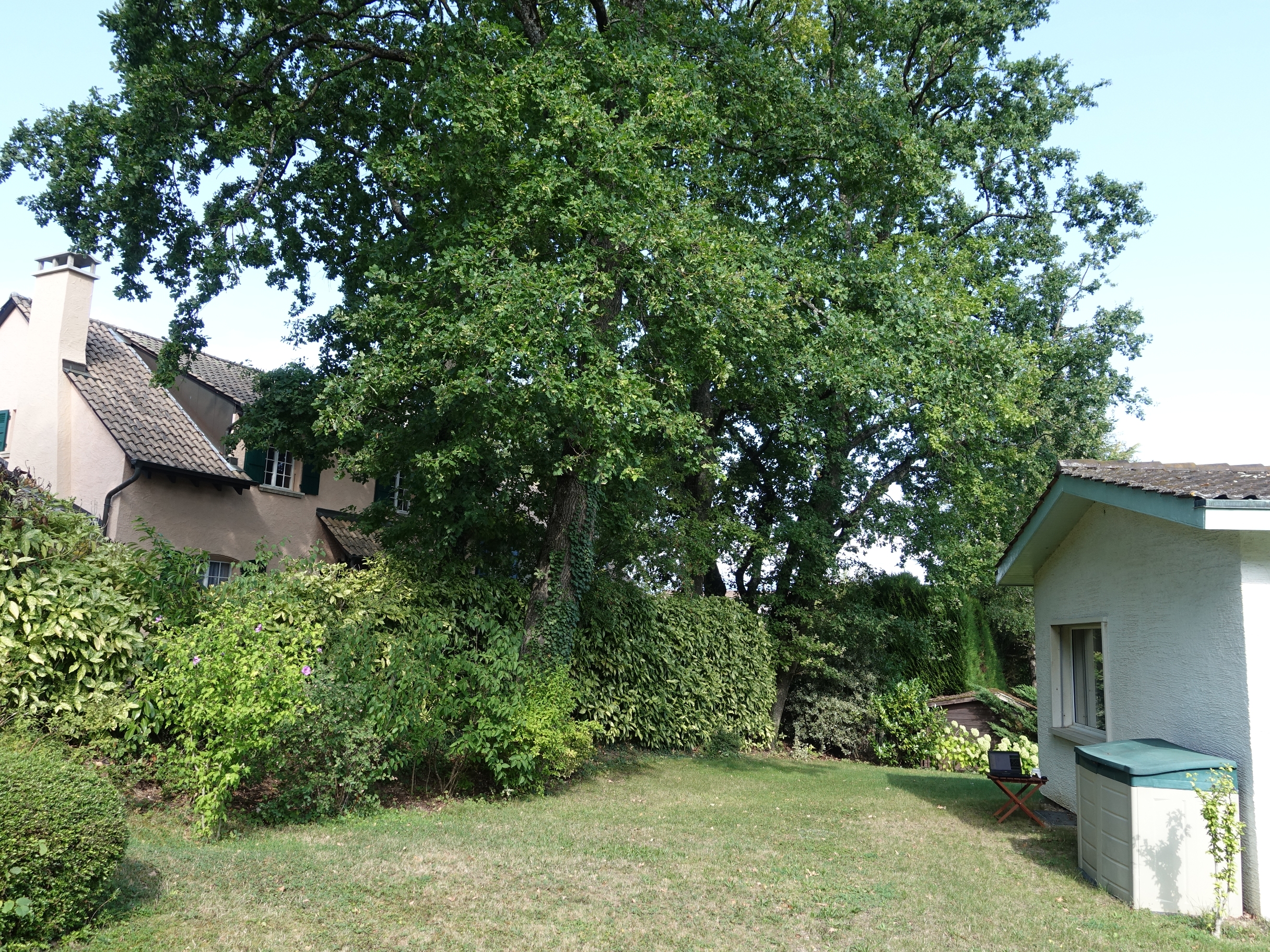
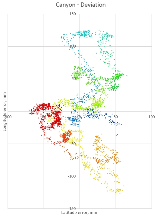
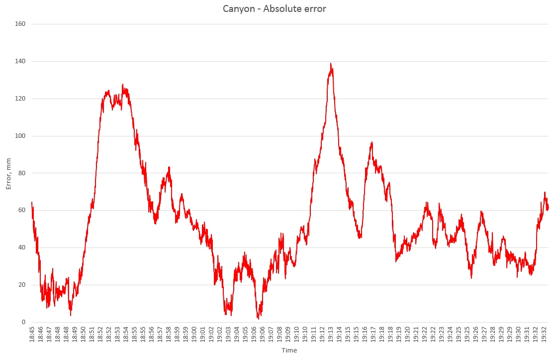
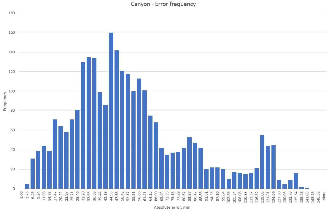
Canyon test
The receiver is in a NE-SW canyon between two houses with heavy canopy:

The wide-angle lens gives the impression that there is a wide view towards the camera. This is not the case, the two houses’ walls are almost parallel, some 12 metres apart and the canopy almost reaches to above the camera.
The receiver never achieves Fixed mode. The 3σ CEP is 135 mm.
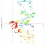
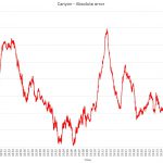
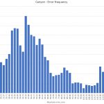
The error and histogram are noisier and the canyon effect is clear in the deviation map, where the longitude errors are double the latitude errors, again due the the constellation geometry (few SVs NE and SW):
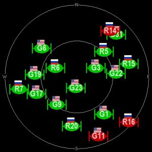
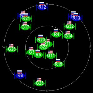
Mobile test
I walked around the garden, pausing 10 seconds at each of the SKYNNN points to hold the GPS at a marked position.
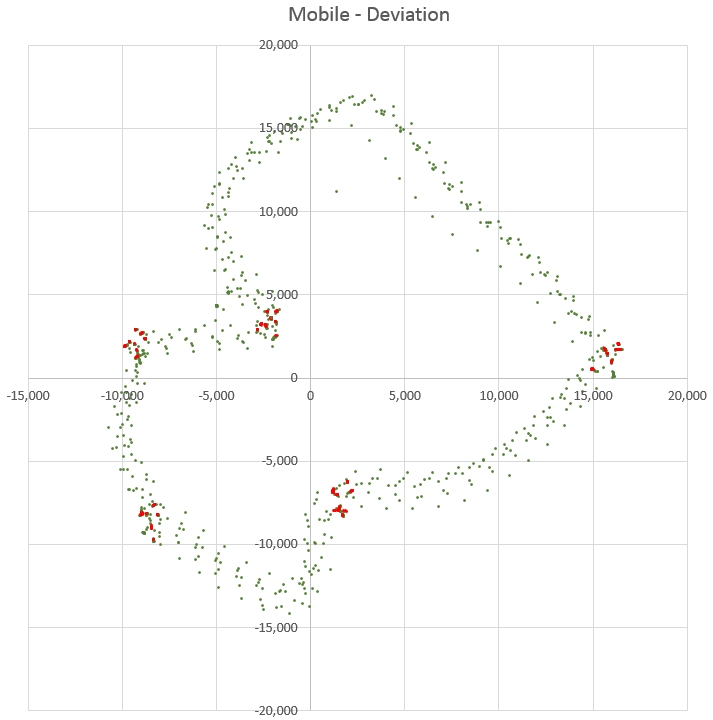
The red points are the 9 nearest points to the average of each location.
The receiver was in Fixed mode 7% of the time.
The average position error when moving is 19 mm.
Lessons learned
Here are some tips which might be useful to those envisaging the C98-M8P solution.
Status
The status bar at the bottom-right of U-Centre is very helpful:

From left to right:
- Version of connected GPS
- Port, if a GPS is connected
- File currently open (recording or replay)
- The last message-type received. This is particularly useful to confirm that you are receiving RTCM messages, where you will see the field display UBlox-NMEA-RTCM in quick succession.
- Elapsed time
- TOD
Antennæ
UBlox stress repeatedly that the solution’s accuracy depends on the antenna quality. I verified this and was unable to get the receiver to converge to ‘fixed’ mode (the highest accuracy) with the supplied patch antennas, so I bought a pair of Garmin GA38.
Startup accuracy
I was disappointed with my initial tests, until it dawned on me that the receiver needs quite a while to converge on the optimal solution. Here is an error plot on power-up:
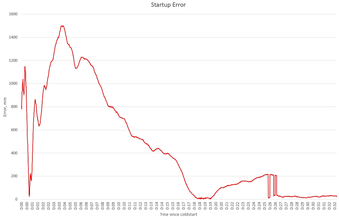
After 52 seconds the error is momentarily down to 24 mm, but it quickly rises to 1’400 mm, thereafter gradually getting close to zero over the next 13 minutes. It again wanders up to 200 mm over 5 minutes and achieves first Fix at 25:54. It finally alternates between Fix and Float for a couple of minutes before permanently settling to Fixed at 26:47. All this is perfectly reasonable, given the calculations involved.
The takeaway is that you should give the receiver half an hour to warm-up before you can expect accurate results. Note also that seeing it switch to Fixed is not a guarantee that it has completely settled.
Fixed .vs. Float
It is apparent from the Sky090 test results that Fixed mode is an indicator of better quality but not a guarantee. All that can be said is that if the quality is 4 or 5, it’s RTK; lower values are standard GPS.
Power
On a 7.45 V battery, the base station consumes ~0.077 A = 0.573 W.
At 12.58 V, the rover consumes 0.066 A = 0.83 W.
So the evaluation board seems to use a linear regulator and I imagine that a non-negligible amount of that power goes to the blinking LEDs.
At closer to 3.5 V, you can assume a power consumption base or rover << 0.5 W.
Interference
As I discovered in the Sky360 test, unexpected interference can cause the unit to lose the RTK solution. The application can detect when this occurs by observing a Quality < 4; the consequence is that the position accuracy will be significantly degraded for the following 20 minutes.
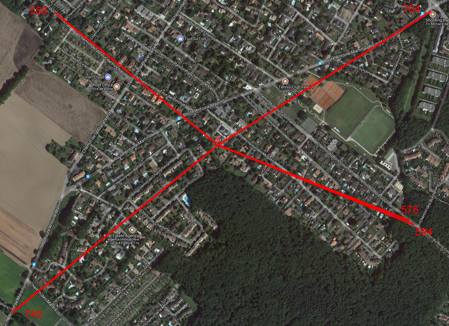
Baseline & Radio range
Although not relevant for my use-case, I nonetheless tested the maximum baseline distance by driving away from the base station with the unit on my dashboard.
The receiver was never in Fixed mode in the car and lost Float mode (falling back to a 3D fix) between 576 and 745 metres away from the base. The distances to the loss points are in red:

(The terrain in my area is almost perfectly flat.)
This limitation is certainly not due to the (amazing) UHF radio, I drove 13 kilometres away from the base and the RTCM stream arrived faultlessly during the whole journey.
Survey-In
There seems to be some confusion about precision and accuracy of the base station. Given the non-Gaussian nature of GPS measurements, acquiring a TRUE position (whatever that means) by averaging would take weeks (months?) simply because the precision of the average depends on the ‘Gausian-ness’ of the data. The base station’s absolute coordinates, insofar as they are within metres of the truth, are irrelevant because the base transmits only satellite relative errors to the rover. The rover uses these relative numbers to adjust it’s solution; the accuracy of the result is not contingent on the precision of the base. Given that the satellites are ~20’000 Km away, a rover-base distance < 100 KM means that they both see identical distortions and this is why RTK baselines are generally recommended to be less than 50-100 Km.
If follows that it is perfectly acceptable to perform a Survey-In in 1 minute with an error of 5 metres, your accuracy will be no better than surveying for an hour with a 30cm error. That said, expect a survey-in of 1 metre to take about 10 minutes.
Deviation Map
You can scroll in and out with the mouse-wheel, but the minimum is 1 metre. To scroll in more, hold the Shift key, whence you can scroll in to a diameter to 20 cm.
Radio baud rate
The default baud rate is 19’200. Initially, I couldn’t get the RTCM messages to flow and finally discovered an error message: “GNTXT More than 100 frame errors, UART RX was disabled”. Reducing the baud rate to 9’600 fixed this, with no apparent consequences.
Summary
What does all this mean in layman’s terms?
Assuming the following conditions:
- Urban environment
- Reasonable antenna
- 50 cm off the ground
- During one hour, from a known truth position
I can make the following assertions about the accuracy and precision:
Accuracy. The error of the reported position will be less than 28 mm from the truth 99.73% of the time. In an urban canyon the error rises to 68 mm and with only 25% of the sky visible 93mm:
On average, you will get one reading worse than these values every 6 minutes.
Precision. Will never be worse than the precision of your base station ±356 mm (the radius of the 24-hour CEP).
Conclusions
The promised accuracy is indeed ‘stunning’.
When combined with a TOF camera, the accuracy of a few centimetres is more than adequate for the mower I am building, so I’m perfectly satisfied with it.
That said, the limitations I discovered preclude this solution in some other use-cases that come to mind. Both UAV and farming applications require a much longer baseline and the inability to maintain Fixed mode accuracy is a handicap for those needing consistent high accuracy.
If UBlox can fix the baseline limitation and significantly improve the unit’s ability to stay in Fixed mode, this GPS will become a truly amazing feat of engineering.
In the spirit of openness, you are welcome to use the data that gathered, for whatever purpose you see fit. Download here.
I am indebted to my local surveyors, JC Wasser, for explaining the finer points of their art and their advice on how to present my results.

Appendix: Quick Start
If you’d like to try this solution, here’s a summary of the user guide, along with a few tips.
The user guide is clear and setting-up the two stations is easy once you get the hang of u-centre (a nice piece of software, by engineers, for engineers). Assuming a classic setup with a fixed base station, here’s a quick-start guide:
- Download the latest firmware. When you install it (Tools-Firmware Update), it’ll ask for the FIS file which nobody talks about; it’s is hidden away in the u-centre program files, called flash.xml.
- Download the latest version of u-center
Setting up the Base
- The base station needs power. It’ll take if from USB but you’re going to need a source of external power once you’ve finished configuring it. It needs to be between 3.7 and 20 VDC, the + and – signs are on each side of the power connector, you’ll need a magnifying glass to read them.
- Fire up u-centre and connect the card you’ve chosen as base station to a USB port (the cards are identical, it’s your parameters that make them base or rover). Don’t try connecting more than one station to your PC at the same time!
- In what follows, you need to click ‘Send’ in the toolbar at the bottom to transmit you settings over USB to the base station.
- In Message view-UBX-CFG-GNSS, make sure GPS and GLOSSNAS are enabled.
- The base station also needs to know its own location, which it can figure out itself. Expand UBX-CFG-TMODE3, select Mode=1-Survey-In; this is what makes it a base station. The Maximum Observation Time and Required Position Accuracy are actually quite unimportant, because it doesn’t matter what the true latitude and longitude are, so 300 seconds and 3 metres are fine. Assuming you’ve got a good sky view it’ll finish the survey easily in the 5 minutes. If you really insist on better precision, it takes about 10 minutes for an RPA of 1 metre.
- UBX-CFG-MSG and enable F5-05 RTCM3.2 1005, 1077, 1087 and 1230 for UART1. They should all be set to 1 Hz except 1230 where 10 seconds is enough for the GLOSSNAS Code-phase biases.
- UBX-CFG –> PRT set the target=1-UART1, Protocol-in=none, Protocol-out=5-RTCM3 and the baud rate to 9’600. This is saying: Send all RTCM messages to UART1, where they’ll get transmitted on the UHF radio link. I couldn’t get the recommended 19’600 baud rate to work, I kept getting “GNTXT More than 100 frame errors, UART RX was disabled” messages.
- UBX-CFG-CFG and save the configuration. That way, when you power-cycle the base, it will resume operation normally. If you forget this and lose power, go to step 2.
- After a while, perhaps up to half an hour, in the Data View, you’ll see the base station switch to TIME. If it doesn’t, don’t worry, it’ll get there eventually and FLOAT mode already gives good results.
Setting up the Rover
- Unplug the base station and connect the other, rover, station.
- UBX-CFG-PRT set the target=1-UART1, Protocol-in=5-RTCM3, Protocol-out=none and the baud rate to 9’600. This is saying: RTCM messages will coming in on UART1, the UHF radio link.
- After a moment, the rover should start receiving RTCM messages. You won’t see them by default, UBX-CFG-Messages right-click on RTCM and ‘Enable child messages’. Then open the packet console to see them (you won’t see anything in the Text Console).
- Once they’re flowing in, time for a beer, the rover has to converge on the solution and this can also take a while, for me 20 minutes at minimum. You can monitor the convergence progress with UBX-NAV-RELPOSNED, click the ‘Poll’ button bottom-left to update the display if it isn’t enabled. The N and E Relative accuracies will fall gradually and eventually reach 0.01 = 10 centimetres.
- After some time it should switch to Fixed mode. If it doesn’t, don’t worry, as I mentioned in Lessons Learned, Fixed mode is better but not a pre-requisite for decent results.
- Now, and only now, can you make meaningful observations. Restart u-centre (the only way I found to reset the Deviation Map) and View-Deviation Map (F12). Yellow dots = last value, green dots = previous values. To zoom in closer than 1 metre, press Shift whilst scrolling the mouse wheel, the minimum is 20 centimetres.
![\[1000*tan(56/2)=531.7mm\]](http://www.calvert.ch/maurice/wp-content/ql-cache/quicklatex.com-ef77efcfe19702eb7e6c64b199c4dd6e_l3.png "Rendered by QuickLaTeX.com")
![\[((480-1)/2)+(-398.5)/531.7*((480-1)/2)=row\ 60\]](http://www.calvert.ch/maurice/wp-content/ql-cache/quicklatex.com-e3df723ae96bbcf7abaf5ddb2605087a_l3.png "Rendered by QuickLaTeX.com")
![\[Atan(398.5/1000)=-21.7^\circ\]](http://www.calvert.ch/maurice/wp-content/ql-cache/quicklatex.com-114ed79cd069c6d25838d630a076f402_l3.png "Rendered by QuickLaTeX.com")
![\[VFov2=VFov/2\]](http://www.calvert.ch/maurice/wp-content/ql-cache/quicklatex.com-be0fff1d91820dda496838fbd33eda6f_l3.png "Rendered by QuickLaTeX.com")
![\[VSize=Tan(VFov2)*2\]](http://www.calvert.ch/maurice/wp-content/ql-cache/quicklatex.com-eb42f116c7fec982c4a1ef95ba5e8d1a_l3.png "Rendered by QuickLaTeX.com")
![\[VCentre=(Rows-1)/2\]](http://www.calvert.ch/maurice/wp-content/ql-cache/quicklatex.com-95f0da83bf6eb62ad3ecae78db032f98_l3.png "Rendered by QuickLaTeX.com")
![\[VPixel=VSize/(Rows-1)\]](http://www.calvert.ch/maurice/wp-content/ql-cache/quicklatex.com-09ae8167b05622d7f07ef162aee1b4ad_l3.png "Rendered by QuickLaTeX.com")
![\[VRatio=(VCentre-row)*VPixel\]](http://www.calvert.ch/maurice/wp-content/ql-cache/quicklatex.com-29c4a3f95bf599ee89a18d86f05e7c72_l3.png "Rendered by QuickLaTeX.com")
![\[Y=Range*-VRatio\]](http://www.calvert.ch/maurice/wp-content/ql-cache/quicklatex.com-bafa5fbfeb7018f3b346040d36f3c4eb_l3.png "Rendered by QuickLaTeX.com")
![\[VFov2=56/2=28\]](http://www.calvert.ch/maurice/wp-content/ql-cache/quicklatex.com-df5af8854955795a66e97d92340c1ac9_l3.png "Rendered by QuickLaTeX.com")
![\[VSize=Tan(28)*2=1.0634\]](http://www.calvert.ch/maurice/wp-content/ql-cache/quicklatex.com-10d5441912c0fc84ce0907d0c001c39c_l3.png "Rendered by QuickLaTeX.com")
![\[VCentre=(480-1)/2=239.5\]](http://www.calvert.ch/maurice/wp-content/ql-cache/quicklatex.com-ade6ec1c12a1adbdb10cd6a19aca58a6_l3.png "Rendered by QuickLaTeX.com")
![\[VPixel=1.0634/(480-1)=0.00222\]](http://www.calvert.ch/maurice/wp-content/ql-cache/quicklatex.com-e509fd7c99ac59d20affb6128ef363b7_l3.png "Rendered by QuickLaTeX.com")
![\[VRatio=(239.5-60)*0.00222=0.3985\]](http://www.calvert.ch/maurice/wp-content/ql-cache/quicklatex.com-7ed2ca98b44d07afbfad90728073e301_l3.png "Rendered by QuickLaTeX.com")
![\[Y=1000*-VRatio=-398.5 mm\]](http://www.calvert.ch/maurice/wp-content/ql-cache/quicklatex.com-dc173670b9f1a02d2a42e9742654b9fd_l3.png "Rendered by QuickLaTeX.com")