Many traffic-light solutions for Excel exist but all the ones I tried only work for a single light, and I needed an array like this:

I wanted to create a light by simply typing a formula in the light’s cell, with the colour of the light determined by a value in cell elsewhere. The light must change colour as soon as the underlying value changes. This wasn’t as simple to implement as I thought, but in the end a bit of VBA led to this formula :
=trafficlight(Sheet2!B4,Sheet2!B$3,Sheet2!C$3)
and the rest of the lights are created by dragging this formula right and down.
The parameters to the TrafficLight function are:
- The cell containing the value which determines the colour of the light.
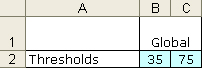
- The threshold to change from red to amber.
- The threshold to change from amber to green.
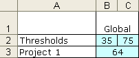
in this example, the Sheet2 looks like this:
Project 1 has a value of 64 and thus is amber.
Here’s a ZIP file with the .XLS and the images project-progress-dashboard, feel free to use it as you see fit.
Notes:
- The red and green images have an exclamation mark and a tick superimposed so that they are recognisable on a black-and-white printout.
- You must keep the 3 GIF files in the same directory as the spreadsheet.
- There is one bug. If you resize a cell containing a light such that the light is no longer contained within the cell’s boundaries, the light will not be deleted when its underlying value changes (you end up with an orphaned light). To fix this, there is a “Remove lights” button; clicking it will delete all images and pressing F9 will re-generate correctly.